Download pdf
Journal link
HAL Link
ARXIV Link
Authors: M. Kobayashi, P. Parnaudeau, F. Luddens, C. Lothodé, L. Danaila, M. Brachet, I. Danaila
Abstract
This paper is concerned with the numerical investigation of Quantum Turbulence (QT) described by the Gross-Pitaevskii (GP) equation. Numerical simulations are performed using a parallel (MPI-OpenMP) code based on a pseudo-spectral spatial discretization and second order splitting for the time integration. We start by revisiting (in the framework of high-performance/high-accuracy computations) well-known GP-QT settings, based on the analogy with classical vortical flows: Taylor-Green (TG) vortices and Arnold-Beltrami-Childress (ABC) flow. Two new settings are suggested to build the initial condition for the QT simulation. They are based on the direct manipulation of the wave function by generating a smoothed random phase (SRP) field, or seeding random vortex rings (RVR) pairs.
The new initial conditions have the advantage to be simpler to implement than the TG and ABC approaches, while generating statistically equivalent QT fields. Each of these four GP-QT settings is described in detail by defining corresponding benchmarks that could be used to validate/calibrate new GP codes. We offer a comprehensive description of the numerical and physical parameters of each benchmark. We analyse the results in detail and present values, spectra and structure functions of main quantities of interest (energy, helicity, etc) that are useful to describe the turbulent flow. Some general features of QT are identified, despite the variety of initial states.
Supplemental material
Context and dimensionless equations
We want to simulate QT flows, in which the total energy of the system can be expressed as: $$ E_T(\psi) = \int \left( \frac{\hbar^2}{2 m} |\nabla \psi|^2 + \frac{g}{2} (|\psi|^2-|\Psi_0|^2)^2 \right) d{\bf x}, $$ where $|\Psi_0|^2=n_0$ is the atomic density of a uniform background. The time evolution of the system is then described by the following GP equation: $$ i \hbar \frac{\partial}{\partial t} \psi({\bf x},t) = \left( - \frac{\hbar^2}{2 m} \nabla^2 + g\left( |\psi({\bf x},t)|^2-|\Psi_0|^2\right) \right) \psi({\bf x},t). $$
We consider the case of a cubic box of length $L$, with periodic boundary conditions. To perform numerical simulations, we use dimensionless equations. In all the following, we take the scaling (see $\S$4.1) $$ {\bf x} \rightarrow \frac{\bf x}{L_{ref}}, \quad {t} \rightarrow \frac{v_{ref}\;t}{L_{ref}}, \quad \psi \rightarrow \frac{\psi}{\sqrt{n_0}}. $$
$L_{ref}$ and $v_{ref}$ are the refence length and velocity respectively. We use $L_{ref}=\dfrac{L}{2\pi}$ so that numerical simulations are performed in a cubic box of size $2\pi$. Furthermore, we introduce $$ \alpha = \frac{\hbar}{2mL_{ref}v_{ref}},\qquad \beta = \frac{gn_0L_{ref}}{\hbar v_{ref}},\qquad M_{ref} = \frac{v_{ref}}{c}, $$ where $c$ is the speed of sound. In all the presented computations, $M_{ref}$ (reference Mach number) is set to $\dfrac12$, i.e. the product $\alpha\beta$ is always equal to 2. The dimensionless GPE then reads: $$ i\partial_t \psi = \left(-\alpha\nabla^2 + \beta\left(|\psi|^2-1\right)\right)\psi, $$ We also rescale the total energy with the reference energy $E_{ref} = \rho_0 v_{ref}^2 L^3$, so that the dimensionless energy is: $$ E(\psi) = \frac{2\alpha}{(2\pi)^3}\int \left( \alpha|\nabla\psi|^2 + \frac{\beta}{2}\left(|\psi|^2-1\right)^2\right) d{\bf x}. $$
QT from different initial conditions
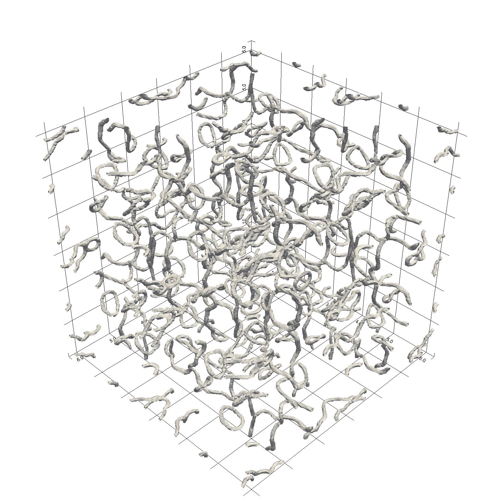
The following movies show the time evolution of the quantum vortices for different kinds of initial conditions. The analysis of the spectra or structure functions of the solution $\psi$ shows similarities between all the different cases.
In each case, we represent the iso-surface of low density $\rho=0.4$. Usually, this is enough to capture the vortex structures. In the SRP case, we add a visualization with gnuplot where only the vortices are computed by detecting phase jump on a cell face.
| Test Case | Parameters (as in paper) | Movie |
|---|---|---|
 |
TG_a \begin{align*} \alpha &= 0.05 \\ \beta &= 40 \\ N_x &= 128 \\ \delta t &= 1.25e-3 \\ T_f &= 12 \\ [\gamma_d/4] &= 3 \end{align*} | Taylor-Green initial condition ➟ Download/Watch movie (2 panels) Or movie with 4 panels (for symmetries) ➟ 4 panels |
 |
ABC_b \begin{align*} \alpha &= 0.025 \\ \beta &= 80 \\ N_x &= 256 \\ \delta t &= 4.0e-4 \\ T_f &= 10 \\ (A,B,C) &= (0.9; 1; 1.1)/\sqrt{3} \end{align*} | ABC initial condition ➟ Download/Watch movie Or vortex visualization with Gnuplot ➟ vortices with gnuplot |
 |
SRP_a (no vortex at $t=0$, as shown in the picture) \begin{align*} \alpha &= 0.05 \\ \beta &= 40 \\ N_x &= 128 \\ \delta t &= 1/1024 \\ T_f &= 8 \\ K &= 8\pi \\ N_r &= 4 \end{align*} | Smooth random phase initial condition ➟ Download/Watch movie Or vortex visualization with Gnuplot ➟ vortices with gnuplot |
 |
RVR_b \begin{align*} \alpha &= 0.025 \\ \beta &= 80 \\ N_x &= 256 \\ \delta t &= 1/2048 \\ T_f &= 8 \\ N_V &= 400 \\ R &= \pi/2 \\ d &= \pi \end{align*} | Random vortex rings initial condition ➟ Download/Watch movie |
ARGLE procedure
One way to compute a suitable initial condition for QT is to find a stationary state that mimics a classical flow with prescribed velocity ${\bf v}_{ext}$, see $\S$ 4.2. Using a pseudo-time $\tau$, this amounts to solve $$ \frac{\partial}{\partial\tau}\phi = \left(\alpha\nabla^2 - i {\bf v}_{ext} \cdot\nabla - \frac{ |{\bf v}_{ext}|^2 }{4\alpha} + \beta - \beta|\phi|^2\right)\phi $$ until a steady state is reached.
The following movies show the (pseudo-)time evolution of $\phi$ during the ARGLE procedure, for TG and ABC cases. They illustrate the preparation of the initial condition of QT simulations shown above.
| Test Case | Parameters | Movie |
|---|---|---|
 |
TG_aIT \begin{align*} \alpha &= 0.05 \\ \beta &= 40 \\ N_x &= 128 \\ \delta \tau &= 1.25e-2 \\ \tau_f &= 60 \\ [\gamma_d/4] &= 3 \end{align*} | Taylor-Green initial condition ➟ Download/Watch movie (2 panels) Or movie with 4 panels (for symmetries) ➟ 4 panels |
 |
ABC_bIT \begin{align*} \alpha &= 0.025 \\ \beta &= 80 \\ N_x &= 256 \\ \delta\tau &= 2.0e-3 \\ \tau_f &= 30 \\ (A,B,C) &= (0.9; 1; 1.1)/\sqrt{3} \end{align*} | ABC initial condition Animation with 3 frames only ➟ Download/Watch animation Or vortex visualization with Gnuplot ➟ vortices with gnuplot |