Download pdf
HAL Link
ARXIV Link
Authors: S. Laurent, P. Parnaudeau, F. Chevy, I. Danaila
Abstract
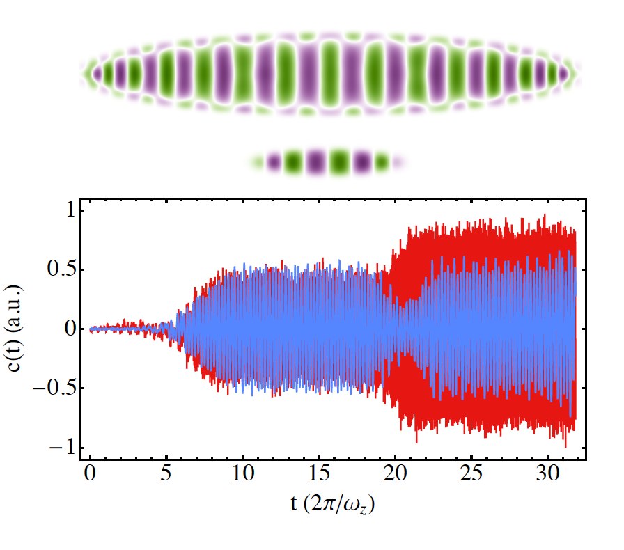
We study the coupling between modes of two harmonically trapped counterflowing superfluids. Using a combination of analytical and numerical approaches, we exhibit two different excitation mechanisms leading to distinct threshold velocities for the onset of dissipation. In addition to the parametric pair production present in homogeneous systems, we show that density inhomogeneities allow for a Landau-like decay mechanism.
Supplemental material
We recall the system of coupled Gross-Pitaevskii equations used in the paper to describe the interaction of two counterflowing superfluids: $$ \displaystyle i \hbar \frac{\partial \psi_1}{\partial t}= \displaystyle \left[-\frac{\hbar^2}{2m_1} \nabla^2 + U({\bf r}) + N_1 g_{11} |\psi_1|^2 + N_2 g_{12}|\psi_2|^2\right]\psi_1,$$ $$ \displaystyle i \hbar \frac{\partial \psi_2}{\partial t} =\displaystyle \left[-\frac{\hbar^2}{2m_2} \nabla^2 + U({\bf r}) + N_1 g_{21} |\psi_1|^2 + N_2 g_{22} |\psi_2|^2 \right]\psi_2. $$ with $$ U({\bf r})=\frac{1}{2}m_2\left[\omega_\perp^2(x^2+y^2)+\omega_z^2z^2\right]. $$
Numerical simulations are performed using dimensionless variables. We take the usual scaling: $$ {\bf x} \rightarrow \frac{\bf x}{x_s}, \quad {t} \rightarrow \frac{t}{t_s}, \quad u_1 = \frac{{\psi_1}}{ x_s^{-3/2}}, \quad u_2 = \frac{{\psi_2}}{ x_s^{-3/2}}. $$ with $$ t_s =\frac{1}{\omega}, \quad x_s = a_{ho}, \,\, a_{ho}=\sqrt{\frac{\hbar}{m \omega}}. $$ The scaled equation can be written in the following form $$ \displaystyle i \frac{\partial u_1}{\partial t} =\displaystyle \left[-\frac{1}{2 d_1} \nabla^2 + U_a({\bf r}) + \beta_{11} |u_1|^2 + \beta_{12} |u_2|^2\right] u_1, $$ $$ \displaystyle i \frac{\partial u_2}{\partial t} =\displaystyle \left[-\frac{1}{2 d_2} \nabla^2 + U_a({\bf r}) + \beta_{21} |u_1|^2 + \beta_{22} |u_2|^2 \right]u_2, $$ with $u_1$ and $u_2$ normalized to unity: $$ \int_{R^3} |u_1|^2 ={1}, \quad \int_{R^3} |u_2|^2 ={1}. $$ The non-dimensional trapping potential becomes: $$ U_a({\bf r})= \frac{d_2}{2} \left[ \gamma_\perp^2 ({x}^2 + {y}^2) + \gamma_z^2 \left(z-b\right)^2\right] $$ with $b$ (in $a_{ho}$ units) the initial shift of the clouds and $ \gamma_\perp=\left(\frac{\omega_\perp}{\omega}\right), \quad \gamma_z=\left(\frac{\omega_z}{\omega}\right)$. Dimensionless parameters “beta” are expressed by: $$ \beta_{11} = {\displaystyle 4\pi \frac{1}{d_1} \frac{N_1 a_{11}}{a_{ho}}},$$ $$ \beta_{12} = \displaystyle {\displaystyle 2\pi \frac{d_1+d_2}{d_1 d_2} \frac{N_2 a_{12}}{a_{ho}}},$$ $$ \beta_{21} = \displaystyle {\displaystyle 2\pi \frac{d_1+d_2}{d_1 d_2} \frac{N_1 a_{12}}{a_{ho}}},$$ $$ \beta_{22} = \displaystyle {\displaystyle 4\pi \frac{1}{d_2} \frac{N_2 a_{22}}{a_{ho}}}.$$
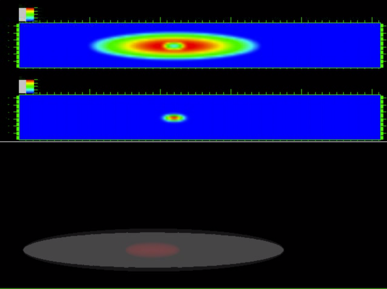
The following movies show the time evolution of the two superfluid clouds by plotting the atomic density in the central longitudinal plane $(z,x)$ (upper panel) and the position of the envelopes of the two clouds (lower panel).
| Initial state ($t=0$) | Parameters | Time oscillations (movie) |
|---|---|---|
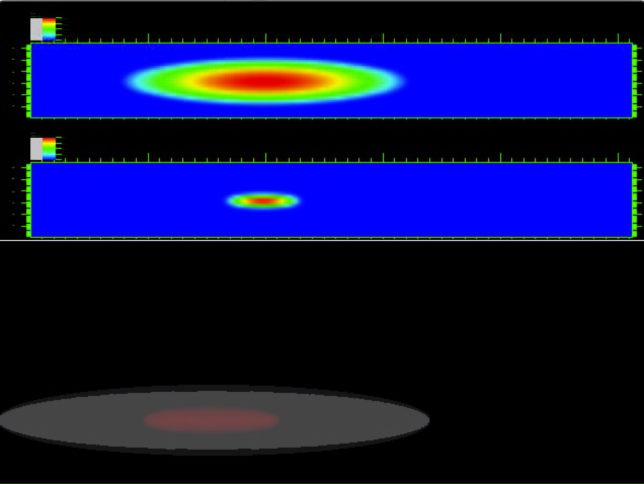 |
$b = 8$ $\beta_{11}$ = 58.934 $\beta_{22}$ = 20621.5 $\beta_{12}$ = 63.8301 $\beta_{21}$ = 2.12767 $\beta_{12}/\beta_{22}=g_{12}/g_{22}= 0.00309$ |
Case-1: parametric instability regime ➟ Download/Watch movie |
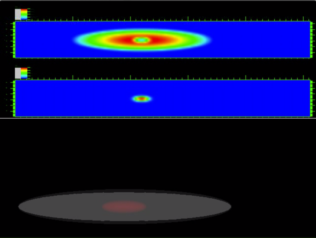 |
$b = 5$ $\beta_{11}$ = 58.938 $\beta_{22}$ = 20621.9 $\beta_{12}$ = 2553.21 $\beta_{21}$ = 85.1069 $\beta_{12}/\beta_{22}=g_{12}/g_{22}= 0.1238$ |
Case-5:
strong linear forcing regime ➟ Download/Watch movie |
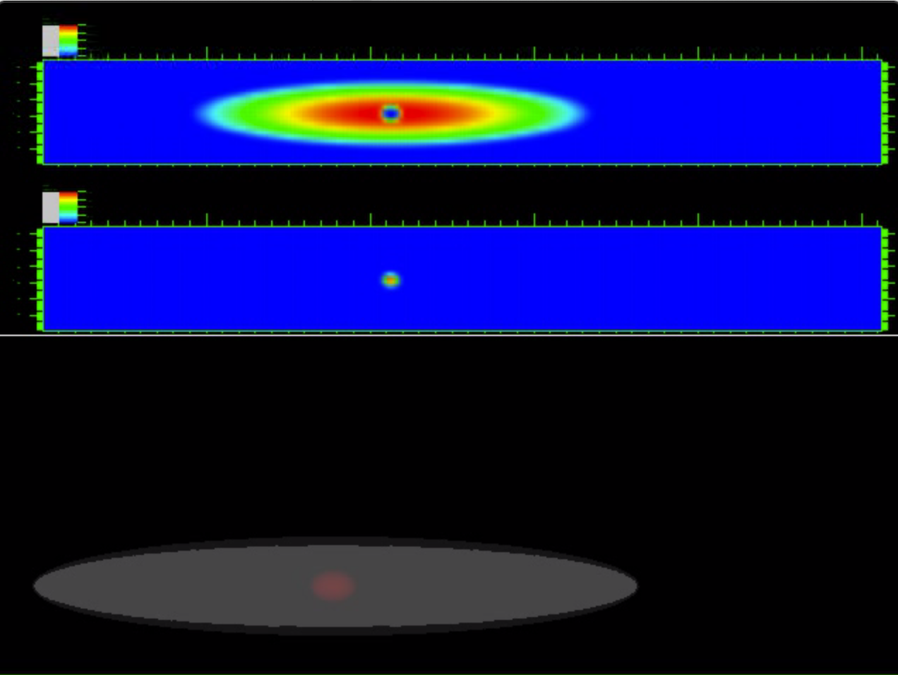 |
$b = 6$ $\beta_{11}$ = 58.939 $\beta_{22}$ = 20621.5 $\beta_{12}$ = 3829.81 $\beta_{21}$ = 127.66 $\beta_{12}/\beta_{22}=g_{12}/g_{22}= 0.1857$ | Case-6: very strong linear forcing regime ➟ Download/Watch movie |
 |
$b = 5$ $\beta_{11}$ = 58.943 $\beta_{22}$ = 20621.1 $\beta_{12}$ = 6000.03 $\beta_{21}$ = 200. $\beta_{12}/\beta_{22}=g_{12}/g_{22}= 0.2909$ |
Case-10 (Part 1): very strong linear forcing regime ➟ Download/Watch movie |
| Case-10 (Part 2) ➟ Download/Watch movie |
||
| Case-10 (Part 3) ➟ Download/Watch movie |
||
| Case-10 (Part 4) ➟ Download/Watch movie |